2. Assignment

- theoritical part

As the 2-dimensional Lebesgue measure of set M is equal to 0.5, the joint density of vector (X, Y) is equal to , where is the identificator of set M. From that, it is easy to find the marginal distributions, which we find as for variable X and for variable Y. For the practical part, we will also need to find the conditional density of X given Y, which is equal to .

As we see, the product of the marginal densities is not equal to the density of the joint distribution, which implies, that the variables X and Y are in fact dependent.

- practical part

In the practical part, we simulated a dataset of 100 observations from the joint distribution mentioned in the theoretical part, using the following code.

Plain version of the code will be present at the end of the page. We can take a look at the basic scatterplot of our dataset with the set M bounded by the red lines.

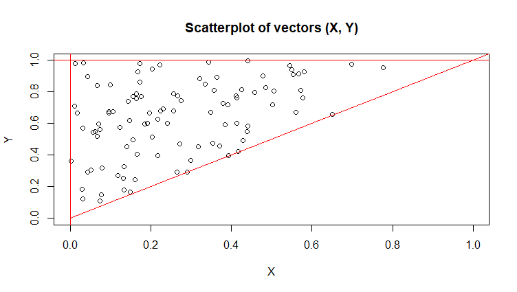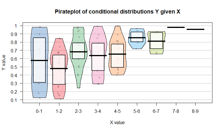
As we see, all the points truly lie inside the set M. To verify the corectness of the distribution, we can study the conditional distribution of X given Y, which should be uniform on the interval (0, Y). The pirateplot below, also showing the estimated densities, does not show any reason to not believe the conditional distribution of X is truly uniform.

We should also study the (conditional) distribution of random variable X, but we can fairly see from the scatterplot, that the resulting conditional densities would look similar to the densities for Y. We can also present some sample characteristics. Sample means for X and Y were equal to 0.26 and 0.64 respectively. The variances were equal to 0.03 and 0.05, covariance was equal to 0.02.

n <- 100

set.seed(1212)

Z <- runif(n)

Y <- sqrt(Z)

Z2 <- runif(n)

X <- Y*Z2

plot(X,Y, main = "Scatterplot of vectors (X, Y)", xlim = c(0,1), ylim = c(0,1))

breks <- seq(0,10,0.1)

lines(x =breks,y= breks, col = "red")

abline( v= 0, col = "red")

abline(h = 1, col = "red")

mean(X)

mean(Y)

cov(cbind(X,Y))

Xbin <- round(X, digits = 1)

plot(Xbin,Y)

Xbin[Xbin == 1] <- 0.9

Xbin <- as.factor(Xbin)

coz <- as.data.frame(cbind(Xbin, Y))

library("yarrr")

pirateplot(Y ~ Xbin, data = coz, xlab = "X value", ylab = "Y value",

main= "Pirateplot of conditional distributions Y given X", inf.method = "iqr", xaxt = "n")

xnames <- c("0-1", "1-2", "2-3", "3-4", "4-5", "5-6", "6-7", "7-8", "8-9" )

axis(side = 1, at = 1:9, labels = xnames)