According to the data from worldpopulationreview.com, states situated in the south of the USA, such as Louisiana or Alabama are leading in homicide rates and firearms death rates in the USA. On the contrary, states in the northeast, such as Maine or New Hampshire, have some of the lowest rates. We can study whether there was a significant difference in crime rates between those two regions in year 1985, using the data from R package SMSdata.
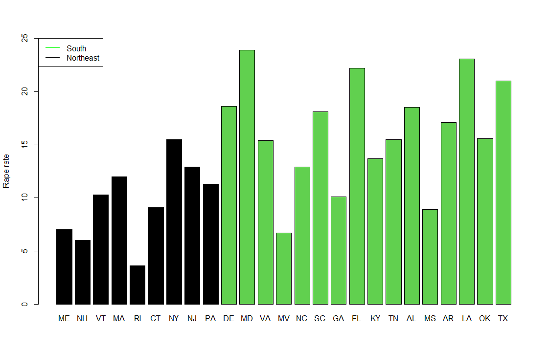
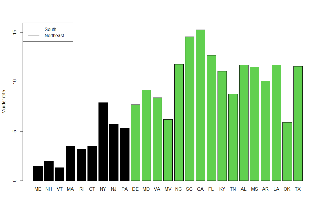
In particular, we will study murder, rape, and robbery rates of states in south an in northeast of USA. In the year 1985, highest murder rate was observed in Georgia, a state in south USA, while the highest robbery rate was observed in New York, state in the northeast. On average, the 16 states in south had higher murder (10.5) and rape (16.3) rates than the 9 states in the northeast (rates 3.8 and 9.7), while the states in northeast had a higher robbery rate (111.0, south = 97.3). We can also formally test, whether there is a statistically significant difference between those rates, indicating that the observed difference isn't just a result of chance.
We will use a two sample hotelling test to test null hypothesis, which assumes that the true expected rates in all 3 categories are the same for both observed regions. Alternative hypothesis will assume, that at least in 1 category the true expected rate is different between the regions. We will not assume, that the variances of rates are the same for both regions. The T squared statistic, which under the null hypothesis has Hotelling distribution with p=3 and n = 11 degrees of freedom, is equal to 105.71. The p-value of the test is about 9*10^6, which means we reject the null hypothesis, proving that at least one of the differences between corresponding rates is statistically significant. Therefore the difference between the regions is not just random, but shows an actual difference in crimes commited, which most likely continued in the following years, possibly even to year 2022.
We proved a difference between at least one of the rates, but the test itself doesn't say, which of the rates are significantly different. We would like to construct confidence intervals, estimating the difference between the expected rates for each of the 3 types of crimes we observed. We can see the table of these intervals below.
|
|
Left bound of CI |
Right bound of CI |
|
Murder rate |
5.53 |
7.97 |
|
Rape rate |
4.40 |
8.77 |
|
Robbery rate |
-74.40 |
47.10 |
Only the confidence interval for robbery rate covers zero, therefore we cannot infer any expected trend in robbery rates for years 1986 and later. For murder and rape rates, the case is different. We expect the average rates in south still exceed the rates in the northeast in following years, but the interval doesn't tell us what the actual differences in next year may be, rather it tells us how the region rates averaged over more years could look like.